Download Skeletons

Version update

This tutorial has recently been updated to materialization version 1412 (from 1300).

We have released a new public version 1412, as part of our quarterly release schedule. See details at Release Manifests: 1412.

Connected morphological representations: skeletons

Often in thinking about neurons, you want to measure things along a linear dimension of a neuron.

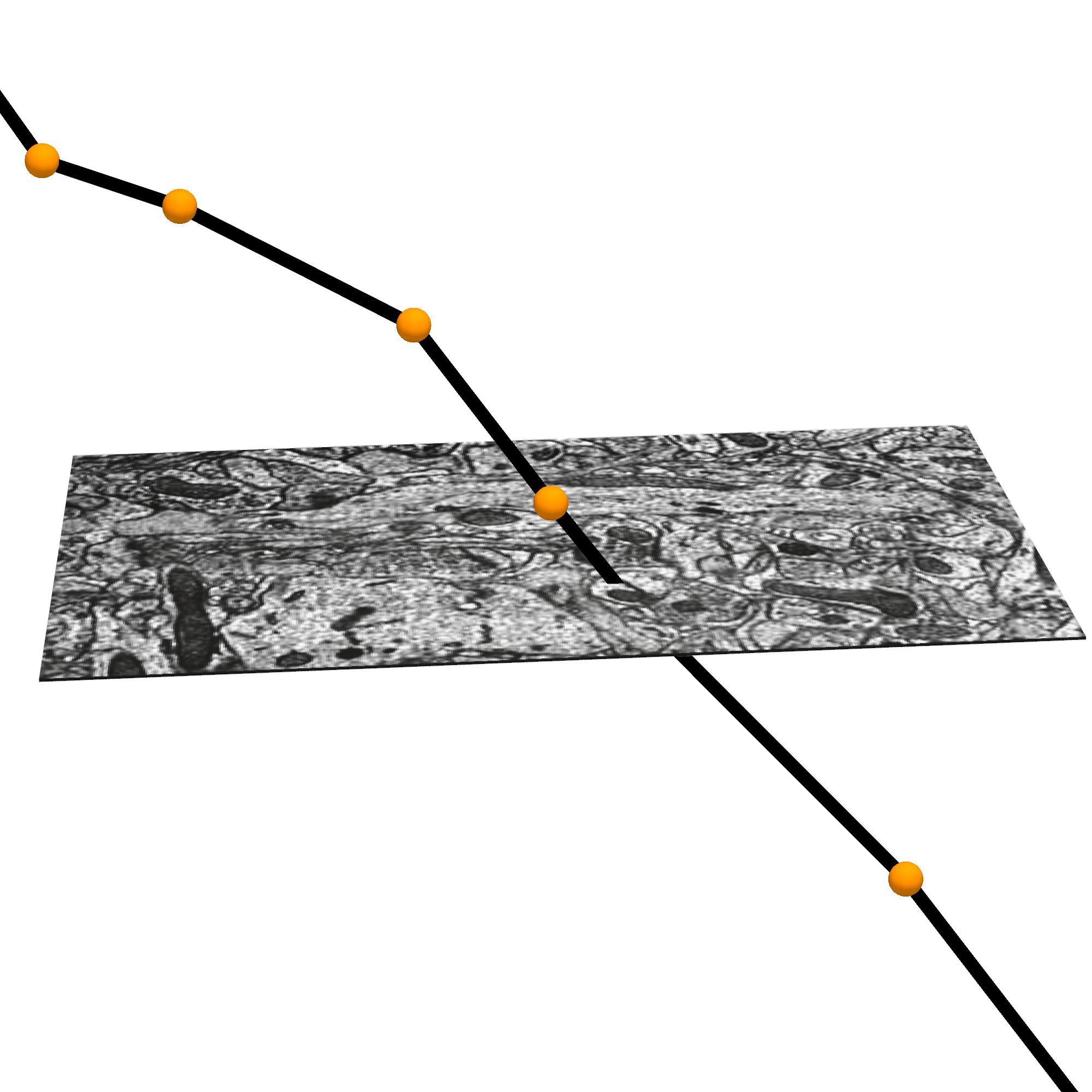
However, the segmentation and meshes are a full complex 3d shape that makes this non-trivial. There are methods for reducing the shape of a segmented neuron down to a linear tree like structure usually referred to as a skeleton. We have precalculated skeletons for a large number of cells in the dataset, and make the skeleton generation available on our server, on demand.

The meshes that one sees in Neuroglancer are available to download through the python client cloud-volume, and can be loaded for analysis and visualization in other tools.

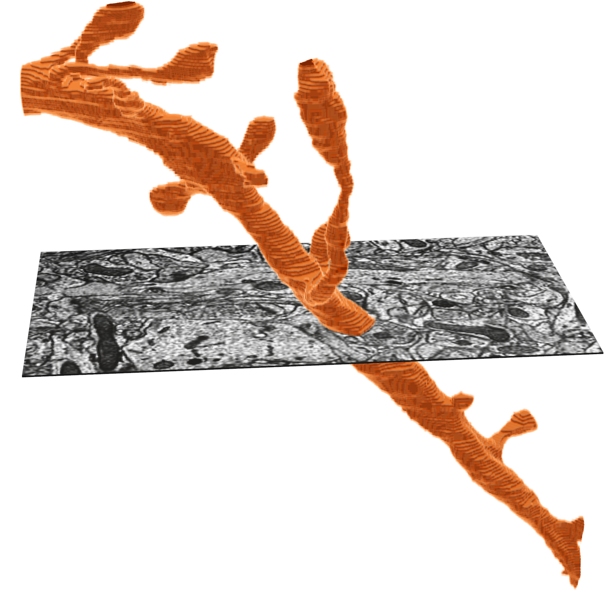
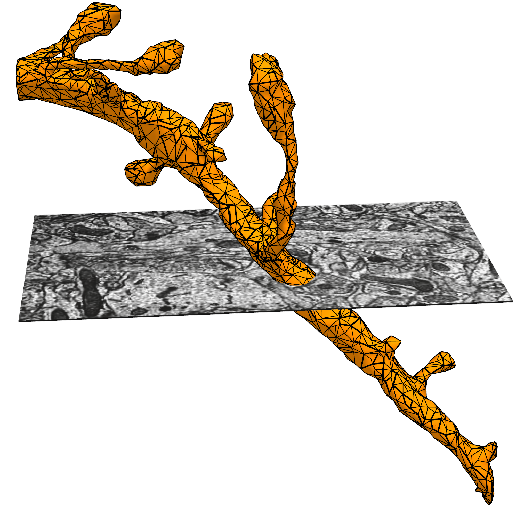
The MICrONS data can be representing and rendered in multiple formats, at different levels of abstraction from the original imagery.

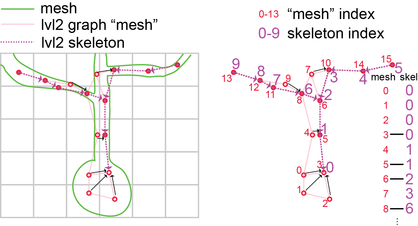
What is a Precomputed skeleton?

These skeletons are stored in the cloud as a bytes-IO object, which can be viewed in Neuroglancer, or downloaded with CAVEclient.skeleton module. These precomputed skeletons also contain annotations on the skeletons that have the synapses, which skeleton nodes are axon and which are dendrite, and which are likely the apical dendrite of excitatory neurons.

For more on how skeletons are generated from the mesh objects, and additional tools for generating, cacheing, and downloading meshes, see the Skeleton Service documentation

CAVEclient to download skeletons

Retrieve a skeleton using get_skeleton(). The available output_formats (described below) are:

dict containing vertices, edges, radius, compartment, and various metadata (default if unspecified)
swc a Pandas Dataframe in the SWC format, with ordered vertices, edges, compartment labels, and radius.

Note: if the skeleton doesn’t exist in the server cache, it may take 20-60 seconds to generate the skeleton before it is returned. This function will block during that time. Any subsequent retrieval of the same skeleton should go very quickly however.

Initial Setup

Before using any programmatic access to the data, you first need to set up your CAVEclient token.

from caveclient import CAVEclient
import numpy as np
import pandas as pd

client = CAVEclient("minnie65_public")

# specify the materialization version, for consistency across time",
client.version = 1412

# Example: pyramidal cell in v1412
example_cell_id = 864691135572530981

sk_df = client.skeleton.get_skeleton(example_cell_id, output_format='swc')

sk_df.head()

	id	type	x	y	z	radius	parent
0	0	1	1365.120	763.456	812.60	3.643	-1
1	1	3	1368.200	755.760	811.24	0.300	0
2	2	3	1368.200	758.552	811.68	1.915	1
3	3	3	1368.200	758.560	812.12	1.915	2
4	4	3	1368.192	758.560	812.44	2.815	3

Skeletons are “tree-like”, where every vertex (except the root vertex) has a single parent that is closer to the root than it, and any number of child vertices. Because of this, for a skeleton there are well-defined directions “away from root” and “towards root” and few types of vertices have special names:

You can see these vertices and edges represented in the alternative dict skeleton output.

sk_dict = client.skeleton.get_skeleton(example_cell_id, output_format='dict')

sk_dict.keys()

dict_keys(['meta', 'edges', 'mesh_to_skel_map', 'root', 'vertices', 'compartment', 'radius'])

Alternately, you can query a set of root_ids, for example all of the proofread cells in the dataset, and bulk download the skeletons

prf_root_ids = client.materialize.tables.proofreading_status_and_strategy(
    status_axon='t').query()['pt_root_id']
prf_root_ids.head(3)

0    864691135308929350
1    864691135163673901
2    864691136812081779
Name: pt_root_id, dtype: int64

all_sk_dict = client.skeleton.get_bulk_skeletons(
    prf_root_ids.head(3), 
    generate_missing_skeletons=True,
    output_format='dict',
    skeleton_version=4)

all_sk_dict.keys()

dict_keys(['864691135308929350', '864691135163673901', '864691136812081779'])

all_sk_dict['864691135308929350'].keys()

dict_keys(['meta', 'edges', 'mesh_to_skel_map', 'root', 'vertices', 'compartment', 'radius', 'lvl2_ids'])

convert dictionary to meshwork skeleton

We use the python package Meshparty to convert between mesh representations of neurons, and skeleton representations.

See Download Meshes | MeshParty for more details.

Converting the pregenerated skeleton sk_dict to a meshwork object sk converts the skeleton to a graph object, for convenient representation and analysis.

from meshparty.skeleton import Skeleton

sk = Skeleton.from_dict(sk_dict)

Plot with skeleton_plot

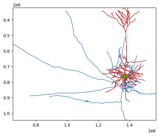
Our convenience package skeleton_plot renders the skeleton in aligned, 2D views.

pip install skeleton_plot

Our convenience package skeleton_plot renders the skeleton in aligned, 2D views, with the compartments labeled in different colors. Here, dendrite is red, axon is blue, and soma (the root of the connected graph) is olive

from skeleton_plot.plot_tools import plot_skel

plot_skel(sk=sk,
          invert_y=True,
          pull_compartment_colors=True,
          plot_soma=True,
         )

Download or generate skeletons with `pcg_skel`

pcg_skel is a package used to rapidly build neuronal skeletons from electron microscopy data in the CAVE ecosystem. It integrates structural data, connectivity data, and local features stored across many aspects of a CAVE system, and creates objects as Meshparty meshes, skeletons, and MeshWork files for subsequent analysis.

By harnessing the way the structural data is stored, you can build skeletons for even very large neurons quickly and with little memory use.

To install pcg_skel, use pip.

pip install pcg_skel

By loading a skeleton as a meshwork skeleton, you can easily ‘rehydrate’ the mesh features of the neuron (annotations such as synapses and compartment labels) and MeshParty functions (such as masking and pathlength)

from pcg_skel import get_meshwork_from_client

sk_mesh = get_meshwork_from_client(example_cell_id,
                                   client=client,
                                   synapses=True,
                                   restore_graph=True,
                                   restore_properties=True,
                                   skeleton_version=4,
)
sk_mesh

<meshparty.meshwork.meshwork.Meshwork at 0x29f79b4cc50>

Branch point: vertices with two or more children, where a neuronal process splits.
End point: vertices with no childen, where a neuronal process ends.
Root point: The one vertex with no parent node. By convention, we typically set the root vertex at the cell body, so these are equivalent to “away from soma” and “towards soma”.
Segment: A collection of vertices along an unbranched region, between one branch point and the next end point or branch point downstream.

MeshWork skeletons represent the neuron as a graph, with tools and properties to utilize the skeleton csgraph.

Properties

branch_points: a list of skeleton vertices which are branches
root: the skeleton vertice which is the soma
distance_to_root: an array the length of vertices which tells you how far away from the root each vertex is
root_position: the position of the root node in nanometers
end_points: the tips of the neuron
cover_paths: a list of arrays containing vertex indices that describe individual paths that in total cover the neuron without repeating a vertex. Each path starts at an end point and continues toward root, stopping once it gets to a vertex already listed in a previously defined path. Paths are ordered to start with the end points farthest from root first. Each skeleton vertex appears in exactly one cover path.
csgraph: a scipy.sparse.csr.csr_matrix containing a graph representation of the skeleton. Useful to do more advanced graph operations and algorithms. https://docs.scipy.org/doc/scipy/reference/sparse.csgraph.html
kdtree: a scipy.spatial.ckdtree.cKDTree containing the vertices of skeleton as a kdtree. Useful for quickly finding points that are nearby. https://docs.scipy.org/doc/scipy/reference/generated/scipy.spatial.cKDTree.html

Methods

path_length(paths=None): the path length of the whole neuron if no arguments, or pass a list of paths to get the path length of that. A path is just a list of vertices which are connected by edges.
path_to_root(vertex_index): returns the path to the root from the passed vertex
path_between(source_index, target_index): the shortest path between the source vertex index and the target vertex index
child_nodes(vertex_indices): a list of arrays listing the children of the vertex indices passed in
parent_nodes(vertex_indices): an array listing the parent of the vertex indices passed in

You access each of these properties and methods with sk.skeleton.* Use the ? to read more details about each one

Annotation properties

sk.anno has set of annotation tables containing some additional information for analysis. Each annotation table has both a Pandas DataFrame object storing data and additional information that allow the rows of the DataFrame to be mapped to mesh and skeleton vertices. For the neurons that have been pre-computed, there is a consisent set of annotation tables:

post_syn: Postsynaptic sites (inputs) for the cell
pre_syn: Presynaptic sites (outputs) for the cell
is_axon: List of vertices that have been labeled as part of the axon
lvl2_ids: Gives the PCG level 2 id for each mesh vertex, largely for book-keeping reasons.
segment_properties: For each vertex, information about the approximate radius, surface area, volume, and length of the segment it is on.
vol_prop: For every vertex, information about the volume and surface area of the level 2 id it is associated with.

To access one of the DataFrames, use the name of the table as an attribute of the anno object and then get the .df property. For example, to get the postsynaptic sites, we can do:

sk_mesh.anno.post_syn.df.head(3)

	id	size	pre_pt_supervoxel_id	post_pt_supervoxel_id	post_pt_root_id	pre_pt_position	post_pt_position	ctr_pt_position	post_pt_level2_id	post_pt_mesh_ind	post_pt_mesh_ind_filt
0	456611088	5140	113239596703504810	113239596703516355	864691135572530981	[1410648.0, 729000.0, 850240.0]	[1410800.0, 728960.0, 850520.0]	[1410672.0, 728960.0, 850280.0]	185297190741082374	11880	11880
1	460786295	1904	114084296310348680	114084365029814954	864691135572530981	[1434984.0, 737808.0, 794360.0]	[1435488.0, 738120.0, 794120.0]	[1435224.0, 737856.0, 794400.0]	186141959067271764	13325	13325
2	415745273	14532	110214290325399938	110214290325398722	864691135572530981	[1322336.0, 744768.0, 807360.0]	[1322032.0, 744560.0, 807440.0]	[1322120.0, 744656.0, 807360.0]	182271884363039168	3695	3695

However, in addition to these rows, you can also easily get the mesh vertex index or skeleton vertex index that a row corresponds to with nrn.anno.post_syn.mesh_index or nrn.anno.post_syn.skel_index respectively. This seems small, but it allows you to integrate skeleton-like measurements with annotations trivially.

For example, to get the distance from the cell body for each postsynaptic site, we can do:

sk_mesh.distance_to_root(sk_mesh.anno.post_syn.mesh_index)

array([104938.90991211,  90399.17230225,  52673.86270142, ...,
        70199.43048096, 212153.28248978,  91076.815979  ])

Note

Note that the sk.distance_to_root, like all basic meshwork object functions, expects a mesh vertex index rather than a skeleton vertex index.

A common pattern is to copy a synapse dataframe and then add columns to it. For example, to add the distance to root to the postsynaptic sites, we can do:

syn_df = sk_mesh.anno.pre_syn.df.copy()
syn_df['dist_to_root'] = sk_mesh.distance_to_root(sk_mesh.anno.pre_syn.mesh_index)
syn_df.head(3)[['id','size','dist_to_root']]

	id	size	dist_to_root
0	395248437	9532	550625.977657
1	440616430	4432	59338.621429
2	439592768	576	426225.854660

This gives us the path-distance of every synapse from the root in nanometers (nm).

Calculate `path_length()` of axon and dendrite

Given the skeleton graph, it is trivial to estimate the pathlength (sum of all branch lengths) for a neuron:

sk_mesh.path_length() / 1e6 # to convert from nm to mm

np.float32(14.846251)

However, the axon and dendrite compartments differ dramatically in their geometric and physiological properties. You generally will want to treat these seperately.

Fortunately the meshwork skeleton includes annotations as to whether the compartment is likely axon or not:

sk_mesh.anno.is_axon

and you can mask the neuron skeleton by the type of comparment simply by using these annotations as an index:

# Apply a mask to the mesh using the axon labels
sk_mesh.apply_mask(sk_mesh.anno.is_axon.mesh_mask)

print (f'Axon path length is {sk_mesh.path_length() / 1e6} mm')

# Reset the mask
sk_mesh.reset_mask()

print (f'Total path length is {sk_mesh.path_length() / 1e6} mm')

Axon path length is 7.599738121032715 mm
Total path length is 14.846250534057617 mm

Connected morphological representations: skeletons

What is a Precomputed skeleton?

CAVEclient to download skeletons

convert dictionary to meshwork skeleton

Plot with skeleton_plot

Download or generate skeletons with pcg_skel

Annotation properties

Calculate path_length() of axon and dendrite

Download or generate skeletons with `pcg_skel`

Calculate `path_length()` of axon and dendrite