We have begun archiving release versions that are more 1 years old. All publicly released annotation data is available as a static download. See: Access archived data versions for details.
You can continue to access older versions of materialization and segmentation by setting the timestamp argument instead of a version argument. However, fully deprecated tables will no longer be queriable from CAVEclient.
The MICrONS Dataset is public and open access, ready for analysis. But: manual edits to the segmentation continue to improve data quality.
When beginning your analysis in the MICrONS dataset, it is important to understand:
Why the data changes
What types of data change with time
How to set the version for your analysis
How to cross-reference data across time
The data is regularly versioned; that is, a long-term copy of the dataset is made available for users. We highly recommend setting the version or timestamp in your analysis for future consistency.
However, even if you do not set the version, there is a lineage graph of changes to the dataset. Meaning, you can find the past version of your cell, annotation table, mesh, skeleton etc. as long as you know the root id of the object you are interested in–or the date at which you performed an analysis.
Why the data changes
The automatic segmentation from EM imagery to 3D reconstruction was largely effective, and the only way to process data at this scale (The MICrONS Consortium et al. 2025). However, due to imaging defects and the nature of thin, branching axons, the automated methods do make mistakes that have large impacts on the biological accuracy of the reconstructions.
Different aspects of the data require different level of manual intervention. For example, the segmentation methods produced highly accurate dendritic arbors before proofreading, enabling morphological identification of broad cell types. Most dendritic spines are properly associated with their dendritic trunk. Recovery of larger-caliber axons, those of inhibitory neurons, and the initial portions of excitatory neurons was also typically successful. Owing to the high frequency of imaging defects in the shallower and deeper portions of the dataset, processes near the pia and white matter often contain errors. Many non-neuronal objects are also well-segmented, including astrocytes, microglia and blood vessels. The two subvolumes of the dataset were segmented separately, but the alignment between the two is sufficient for manually tracing between them.
Changes to the dataset represent an improvement in accuracy, and reflect an investment in the long-term usefulness of this open-access resource.
What types of data change with time
Proofreading edits to the segmentation change what supervoxels (groups of locally aggregated voxels) are associated with what segmented object. Any time the supervoxel is associated with a different segmented object, all of the ids upstream of that supervoxel will update. In practice, this means the 18-digit segmentation id or pt_root_id of your neuron or microglia or axon etc. will change every time it is proofread.
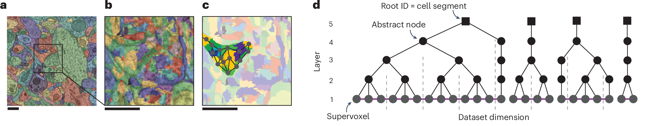
a, Automated segmentation overlaid on EM data. Each color represents an individual putative cell. b, Different colors represent supervoxels that make up putative cells. c, Supervoxels belonging to a particular neuron, with an overlaid cartoon of its supervoxel graph. These data corresponds to the framed square in a and the full panel in b. d, One-dimensional representation of the supervoxel graph. The ChunkedGraph data structure adds an octree structure to the graph to store the connected component information. Each abstract node (black nodes in levels >1) represents the connected component in the spatially underlying graph.
The pt_root_id is always associated with the same collection of supervoxels, and therefore the same mesh and same skeleton. But if that pt_root_id is expired, then you may not find that object in current Annotation Tables, Synapse Connectivity Tables, and Neuroglancer views of the current version of the dataset (default).
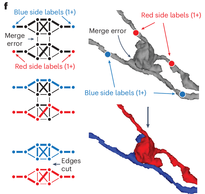
Creating a new pt_root_id for an edited object is the only way to have the flexibility of both merging two or more segments that should be connected (for example: extending an axon) and splitting an object into two, as in the following example:
f, To submit a split operation, users place labels for each side of the split (top right). The backend system first connects each set of labels on each side by identifying supervoxels between them in the graph (left). The extended sets are used to identify the edges needed to be cut with a maximum-flow minimum-cut algorithm.
But this also means we can track the histories of what ids used to be part of which segmented objects, which helps for finding the same cell, axon, or arbitrary segment across time. See Lineage Graphs below for details.
How to set the version of your analysis
Most programmatic access to the CAVE services occurs through CAVEclient, a Python client to access various types of data from the online services.
To initialize a caveclient, we give it a datastack, which is a name that defines a particular combination of imagery, segmentation, and annotation database. For the MICrONs public data, we use the datastack name minnie65_public.
from caveclient import CAVEclientfrom datetime import datetime, timezone# initialize cave clientclient = CAVEclient('minnie65_public')# see the available materialization versionsversions = client.materialize.get_versions()versions.sort()versions
[117, 943, 1300, 1507, 1621, 1718]
And these are their associated timestamps (all timestamps are in UTC):
for version in versions:print(f"Version {version}: {client.materialize.get_timestamp(version)}")
Version 117: 2021-06-11 08:10:00.215114+00:00
Version 943: 2024-01-22 08:10:01.497934+00:00
Version 1300: 2025-01-13 10:10:01.286229+00:00
Version 1507: 2025-07-31 08:10:01.117494+00:00
Version 1621: 2025-11-25 08:10:01.094430+00:00
Version 1718: 2026-03-07 08:10:01.190228+00:00
You can set the overall materialization version for the dataset using client.version. This will ensure all of the subsequent CAVE queries are performed at the same materialization, so you will get consistency between, for example, a cell type query and a synapse query.
# set materialization version, for consistencyclient.version =1300
However, you can also set individual queries to a different version with optional argument materialization_version. For more about table queries, see CAVE Query Cell Types.
You can even do the same thing with an arbitrary timestamp, using optional argument timestamp. However, due to how the ChunkedGraph operates, this will be more time-intensive than looking up a specific materialized version.
Materialization versions expire at regular intervals. Indeed, every version between our major long-term public releases existed at some point, but has since expired.
This does not mean the data from those versions is gone.
It does mean it takes longer to materialize data from that date, because the chunkedgraph has to calculate differences between an extant materialized version and the requested time. In order to materialize data from an expired version, you must set the optional timestamp argument in every query:
# set the timestamp of a version that may or may not existexample_timestamp = datetime(2022, 2, 24, 8, 10, 0, 184668, tzinfo=timezone.utc)# example table querynuc_timestamp = client.materialize.tables.nucleus_detection_v0().query(timestamp=example_timestamp, limit=3000)nuc_timestamp.tail(3)
201 - "Limited query to 3000 rows
id
valid
volume
pt_supervoxel_id
pt_root_id
pt_position
bb_start_position
bb_end_position
2997
225636
True
147.284134
87198969000171523
864691135785277380
[163152, 150992, 17899]
[<NA>, <NA>, <NA>]
[<NA>, <NA>, <NA>]
2998
176753
True
101.935844
82712068070840785
864691136082966797
[130272, 275376, 16387]
[<NA>, <NA>, <NA>]
[<NA>, <NA>, <NA>]
2999
603240
True
217.90834
0
0
[357088, 77280, 20041]
[<NA>, <NA>, <NA>]
[<NA>, <NA>, <NA>]
# example synapse querysyn_timestamp = client.materialize.synapse_query(timestamp=example_timestamp, limit=10)syn_timestamp.head(3)
201 - "Limited query to 10 rows
id
valid
pre_pt_supervoxel_id
pre_pt_root_id
post_pt_supervoxel_id
post_pt_root_id
size
pre_pt_position
post_pt_position
ctr_pt_position
0
106675816
True
84396795031127211
864691136041487043
84467163775312026
864691135785699268
508.0
[142854, 244590, 18572]
[142946, 244642, 18573]
[142890, 244657, 18573]
1
58059862
True
81356507538572374
864691134686377805
81356507538560968
864691136618474893
9516.0
[120492, 136916, 15377]
[120494, 136946, 15368]
[120527, 136988, 15374]
2
334196813
True
103459441311512485
864691136915328110
103389072567345977
864691135467566732
2500.0
[281168, 190270, 25546]
[281088, 190226, 25551]
[281134, 190266, 25552]
Timestamps for all public release versions
Long-term releases are made available for analysis, but are not permanent. You can lookup the timestamp associated with any version here.
CAVEclient materialization version timestamps (as datetime.datetime objects)
Some fully deprecated tables can no longer be accesses from CAVEclient. See Access archived data versions for details.
How to cross-reference across time
Lineage Graphs
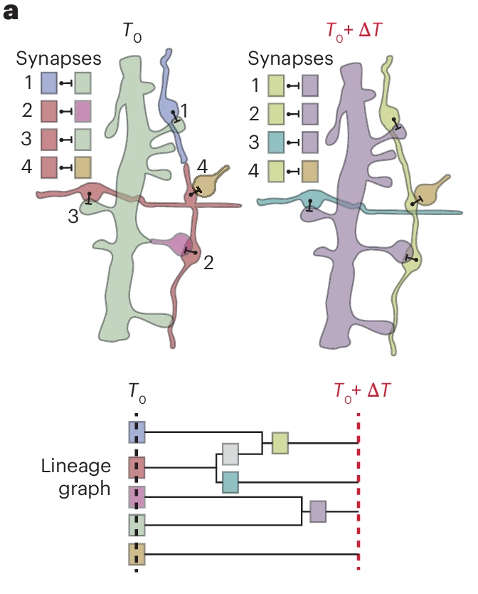
CAVEclient combines materialized snapshots with ChunkedGraph-based tracking of neuron edit histories to facilitate analysis queries for arbitrary time points. The ChunkedGraph tracks the edit lineage of neurons as they are being proofread, allowing us to map any segment used in a query to the closest available snapshot time point. This produces an overinclusive set of segments with which we query the snapshot database.
a, Edits change the assignment of synapses to segment IDs. Each of the four synapses is assigned to the segment IDs (colors) according to the presynaptic and postsynaptic points (point, bar). The identity of the segments changes through proofreading (time passed: ΔT) indicated by different colors. The lineage graph shows the current segment ID (color) for each point in time.
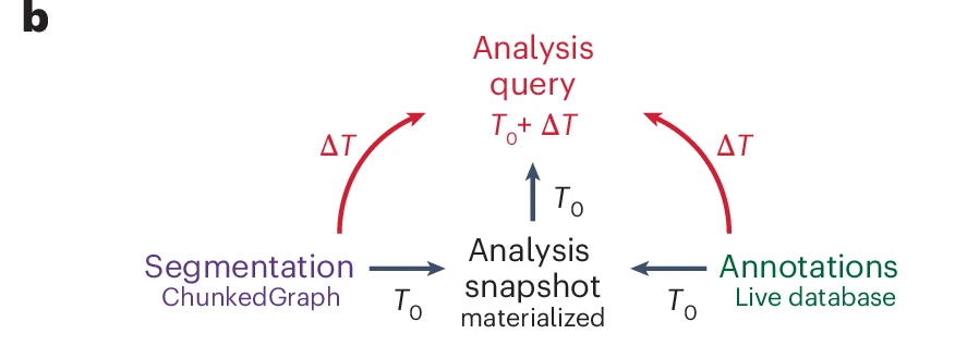
When we query the ‘live’ database for all changes to annotations since the used materialization snapshot and add them to the set of annotations. The resulting set of annotations is then mapped back to the query timestamp using the lineage graph and supervoxel to root lookups and finally reduced to only include the queried set of root IDs.
b, Analysis queries are not necessarily aligned to exported snapshots. Queries for other time points are supported by on-the-fly delta updates from both the annotations and segmentation through the use of the lineage graph.
Most commonly, what you will want is to look-up the current root id for a pt_root_id in a previous analysis. This is not always a trivial thing to do, for example in the case of a multi-soma object that has been manually split. Which of the two new cells was your original cell of interest?
The ChunkedGraph will make its best guess, given supervoxel overlap, with the function suggest_latest_roots()
example_id =864691135919440816# Access the ChunkedGraph service of caveclientclient.chunkedgraph.suggest_latest_roots(example_id, timestamp = client.materialize.get_timestamp())
np.int64(864691134991067002)
Now we have updated pt_root_id for our cell, at the current materialized version.
If you want to run this for a large number of root ids, you can first check if the pt_root_ids are current to your CAVEclient materialization version using is_latest_roots(), and then only update the ids that have expired:
# Check if roots are currentprint(client.chunkedgraph.is_latest_roots(example_id))# See when the id was generated (when the segment was last edited)client.chunkedgraph.get_root_timestamps(example_id)
Using the timestamp argument, you can also lookup the suggested root at any arbitrary time. Here we use the timestamp for a different materialization, verion 943:
Sometimes you may want to check the lineage graph for a cell of interest, to better understand what was edited and why. You can access this and more advanced features from the get_lineage_graph(). See the ChunkedGraph documentation for more use cases.
client.chunkedgraph.get_lineage_graph(example_id)
Static annotations
The CAVEclient Materialization Engine updates segmentation data and creates databases that combine spatial annotation points and segmentation information.
The live database is written to by the Annotation service and is actively managed by the Materialization service to keep root IDs up to date for all BoundSpatialPoints in all tables. Snapshotted databases are copies of a time-locked state of the ‘live’ database’s segmentation and annotation information used to facilitate consistent querying.
This means if you use a static annotation label to index your analysis, for example a nucleus_id or a synapse_id which do not undergo proofreading, you can look up the current pt_root_id at any time by asking CAVEclient to materialize the new segmentation under the static point.
Using our example cell from above, let’s find its nucleus id. If we try to query the nucleus table with the expired id, we will return no result:
This is expected, since the example id is expired at the time of this materialization. Instead, let’s query the version we know this id existed at: version 661
This returns the same pt_root_id as the lineage graph example above. But, it has the benefit of guaranteeing the id belongs to your cell of interest and not an arbitrary chunk of the previous segmented object.
If you are working with a neuron, glial cell, or any cell that has a nucleus detection, we recommend using the nucleus_id as your identifier rather than the pt_root_id.
If you do use pt_root_id, be sure to note the dataset materialization version in your analysis.
Access archived data versions
As the MICrONS dataset matures, we are beginning to deactivate older materialization versions.
All publically released annotation data from these versions remains available, but only as static downloads.
At this time we have allowed the following versions to expire:
Dorkenwald, Sven, Casey M. Schneider-Mizell, Derrick Brittain, Akhilesh Halageri, Chris Jordan, Nico Kemnitz, Manual A. Castro, et al. 2025. “CAVE: Connectome Annotation Versioning Engine.”Nature Methods, April. https://doi.org/10.1038/s41592-024-02426-z.
The MICrONS Consortium, J. Alexander Bae, Mahaly Baptiste, Maya R. Baptiste, Caitlyn A. Bishop, Agnes L. Bodor, Derrick Brittain, et al. 2025. “Functional Connectomics Spanning Multiple Areas of Mouse Visual Cortex.”Nature 640 (8058): 435–47. https://doi.org/10.1038/s41586-025-08790-w.